In the last post, I explained why TikZ is awesome for making plots. One good use case for handmade TikZ plots is to typeset a question like this:

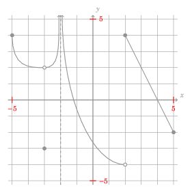
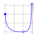
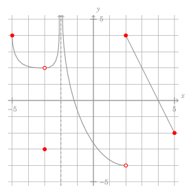
5. (2 points each) A plot of the graph of the function \(f\) is below:

For each of the following expressions, either evaluate the expression or state that it is undefined:

a. \(\lim_{x \rightarrow 2^{-}} f(x)\)

b. \(\lim_{x \rightarrow 2^{+}} f(x)\)

c. \(\lim_{x \rightarrow 2} f(x)\)

d. \(f(2)\)

[. . .]

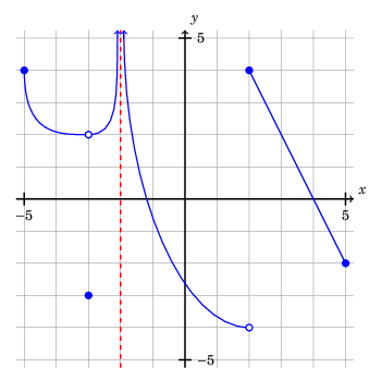
It would be a pain to come up with a formula for a function with the features shown. Before I made these kinds of graphs in TikZ, I would either draw it by hand, or use the drawing features in word-processing software. Drawing by hand is suboptimal, since it requires you to be good at drawing (which I'm not) and the resulting files don't play well with version control. The output from a word-processing software won't play well with version control, either. And using TikZ will make the output automatically have the same font settings as the rest of your document.

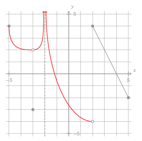
How to create such a plot

Here is the source code for the plot above:

1
2
3
4
5
6
7
8
9
10
11
12
13
14
15
16
17
18
19
20
21
22
23
24
25
26
27
28
29
30
31
32
33
34
35
36
37
38
39
40
41
42
43
44
45
46
47
48
49
50
51
52
53
54
55
56

\documentclass[border=0.25cm]{standalone}

\usepackage{tikz}
\usepackage{fouriernc}

\begin{document}

  \begin{tikzpicture}[scale=0.75]

    \draw[gray] (-5.25, -5.25) grid (5.25, 5.25);

    % x-axis
    \draw[thick, black, ->] (-5.25, 0) -- (5.25, 0)
      node[anchor=south west] {$x$};

    % x-axis tick marks
    \foreach \x in {-5, 5}
      \draw[thick] (\x, 0.2) -- (\x, -0.2)
        node[anchor=north] {\(\x\)};

    % y-axis
    \draw[thick, black, ->] (0, -5.25) -- (0, 5.25)
      node[anchor=south west] {$y$};

    % y-axis tick marks
    \foreach \y in {-5, 5}
      \draw[thick] (-0.2, \y) -- (0.2, \y)
        node[anchor=west] {\(\y\)};

    % graph of function

    \draw[thick, blue, ->] (-5, 4) .. controls (-5, 2) and (-4, 2) .. (-3, 2)
      .. controls (-2.1, 2) and (-2.1, 3) ..
      (-2.1, 5.25);

    \draw[thick, dashed, red] (-2, -5.25) -- (-2, 5.25);

    \draw[thick, blue, <-] (-1.9, 5.25) ..
    controls (-1.9, 0) and (0, -4) .. (2, -4);

    \draw[thick, blue] (2, 4) -- (5, -2);

    \draw[thick, blue, fill=blue] (-5, 4) circle (1mm);

    \draw[thick, blue, fill=white] (-3, 2) circle (1mm);

    \draw[thick, blue, fill=blue] (-3, -3) circle (1mm);

    \draw[thick, blue, fill=white] (2, -4) circle (1mm);

    \draw[thick, blue, fill=blue] (2, 4) circle (1mm);

    \draw[thick, blue, fill=blue] (5, -2) circle (1mm);

  \end{tikzpicture}
\end{document}

Let's go through the construction of this plot. This will also explain the basic syntax of TikZ.

Grid

10

% [...]
\draw[gray] (-5.25, -5.25) grid (5.25, 5.25);
% [...]

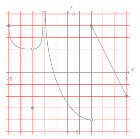
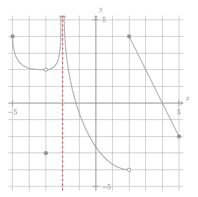
This creates a grid inside the rectangle with opposite corners at \((-5.25, -5.25)\) and \((5.25, 5.25)\). By default, grids in TikZ have their gridlines one unit apart, at integer coordinates. By having the edge of my grid 0.25 units off an integer, I give the subtle impression that the grid extends beyond the graphic. Compare these two grids:

The grid on the left was created with \draw[gray] (-5.25, -5.25) grid (5.25, 5.25); (off-integer edges), while the code on the right was created with \draw[gray] (6, -5) grid (16, 5); (integer edges).

Notice that the grid drawing code is placed first in the tikzpicture. This ensures the grid is drawn first, placing all other elements on top.

Axes

My preference is to have each axis be an arrow with the arrowhead in the positive direction. This is accomplished with:

12
13
14

% [...]
% x-axis
\draw[thick, black, ->] (-5.25, 0) -- (5.25, 0)
  node[anchor=south west] {$x$};
% [...]

21
22
23

% [...]
% y-axis
\draw[thick, black, ->] (0, -5.25) -- (0, 5.25)
  node[anchor=south west] {$y$};
% [...]

The \draw command is used to draw, unsurprisingly. To produce a line segment from \((-5.25, 0)\) to \((5.25, 0)\), one could just do:

% [...]
\draw (-5.25, 0) -- (5.25, 0);
% [...]

You can actually chain line segments together by providing multiple coordinates. For example:

% [...]
\draw (3, 0) -- (4, 2) -- (5, 0) -- (3, 4);
% [...]

Back to the \(x\)-axis, the options [thick, black, ->] produce a thick black line segment with an arrowhead at the end (the last coordinate). But after I draw the line segment, I add some text, using node[anchor=south west] {$x$}. This tells TikZ to place the LaTeX text \(x\) just to the right and above the arrowhead. (It's a bit confusing, but anchor=south west refers to the point of view of the node with the text \(x\), not the point of view of the arrowhead! That is, the arrowhead is southwest of the \(x\).)

Tick marks

16
17
18
19

% [...]
% x-axis tick marks
\foreach \x in {-5, 5}
  \draw[thick] (\x, 0.2) -- (\x, -0.2)
    node[anchor=north] {\(\x\)};
% [...]

25
26
27
28

% [...]
% y-axis tick marks
\foreach \y in {-5, 5}
  \draw[thick] (-0.2, \y) -- (0.2, \y)
    node[anchor=west] {\(\y\)};
% [...]

On each axis are two tick marks. For example, on the \(x\)-axis, I want a tick mark at \((-5, 0)\) and another at \((5, 0)\). Each tick mark is a tick line segment from \((x, 0.2)\) to \((x, -0.2)\), where \(x\) is the horizontal coordinate of the tick mark. I use a for (\foreach) loop to create the tick marks. Below each tick mark is a node with the horizontal coordinate; anchor=north tells TikZ to position the label so that the bottom end of the tick mark (at \((x, -0.2)\)) is north of the label.

Bézier curves

We now start making the plot of the function itself. Two parts are made from Bézier curves, a go-to for making curvy parts.

32
33
34

% [...]
\draw[thick, blue, ->] (-5, 4) .. controls (-5, 2) and (-4, 2) .. (-3, 2)
  .. controls (-2.1, 2) and (-2.1, 3) ..
  (-2.1, 5.25);
% [...]

38
39

% [...]
\draw[thick, blue, <-] (-1.9, 5.25) ..
  controls (-1.9, 0) and (0, -4) .. (2, -4);
% [...]

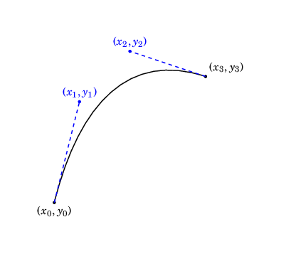
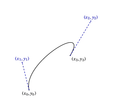
The basic syntax for a Bézier curve in TikZ is \draw (\(x_0, y_0\)) .. controls (\(x_1, y_1\)) and (\(x_2, y_2\)) .. (\(x_3, y_3\)); A Bézier curve is specified by four points:

• A start point (\((x_0, y_0)\) in the diagram below)
• Two control points (\((x_1, y_1)\) and \((x_2, y_2)\) in the diagram below)
• An end point (\((x_3, y_3)\) in the diagram below)

This diagram gives you a sense for how the control points "pull" the curve.

(Side note: Technically, this is a cubic Bézier curve. The curve is parametrized by \[B(t) = (1-t)^3(x_0, y_0) + 3 t(1-t)^2(x_1, y_1) + 3t^2(1-t)(x_2, y_2) + t^3(x_3, y_3), \; 0 \leq t \leq 1.\] For more details, see this article by Bill Casselman, a great expositor on the mathematics of computer graphics.)

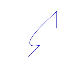
You can even put your Bézier curve in the middle of a draw command, e.g. the following code:

% [...]
\draw[thick, blue] (0, 0) -- (2, 2) .. controls (-3, 1) and (4, 7) .. (5, 8) -- (5, 5);
% [...]

Back to our drawing, consider the left-most Bézier curve, given by:

32
33
34

% [...]
\draw[thick, blue, ->] (-5, 4) .. controls (-5, 2) and (-4, 2) .. (-3, 2)
  .. controls (-2.1, 2) and (-2.1, 3) ..
  (-2.1, 5.25);
% [...]

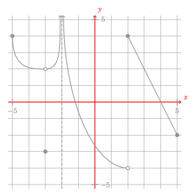
I want a vertical asymptote at \(x=-2\). For readability sake, I actually make the curve end at \((-2.1, 5.25)\). The control point at \((-2.1, 3)\) pulls the curve back and gives the appearance of a vertical asymptote at \(x = -2\). The option -> puts an arrowhead on the end of the curve.

Sidenote: Ensuring that a Bézier curve makes \(y\) a function of \(x\)

It's possible to create a Bézier curve in which \(y\) is not a function of \(x\) (i.e., fails the vertical line test).

With some calculus, one can show that \(x_0 \leq x_1 \leq x_2 \leq x_3\) will ensure this does not happen.¹

Vertical asymptote

I use a thick, dashed, red line segment from \((-2, -5.25)\) to \((-2, 5.25)\) to represent the vertical asymptote at \(x = -2\).

36

% [...]
\draw[thick, dashed, red] (-2, -5.25) -- (-2, 5.25);
% [...]

Line segment part of graph

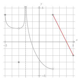
Part of the graph is the line segment from \((2, 4)\) to \((5, -2)\).

41

% [...]
\draw[thick, blue] (2, 4) -- (5, -2);
% [...]

Explicit points

A key advantage for making these graphs using TikZ is to incorporate my visual vocabulary for graphs. I follow the common convention where a filled-in circle indicates a point on the graph, while a hollow circle indicates a point which is not on the graph, e.g. \((-3, 2)\) is not on the graph, while \((-3, -3)\) is.

To accommodate this, we use circles, either filled with the same color as rest of the graph (for points on the graph) or filled with white (to make them hollow). These commands are last, so the white fill punches a hole in the graph.

43
44
45
46
47
48
49
50
51
52
53

% [...]
\draw[thick, blue, fill=blue] (-5, 4) circle (1mm);

\draw[thick, blue, fill=white] (-3, 2) circle (1mm);

\draw[thick, blue, fill=blue] (-3, -3) circle (1mm);

\draw[thick, blue, fill=white] (2, -4) circle (1mm);

\draw[thick, blue, fill=blue] (2, 4) circle (1mm);

\draw[thick, blue, fill=blue] (5, -2) circle (1mm);
% [...]

And with that, our graph is complete!

In the next post, I will explain how to use TikZ to plot graphs of functions defined by a mathematical formula.